Physics Notes: Cosmology
and Black Holes
Lecture by Professor Leonard Susskind
Lecture 9: March 14, 2011 Back to PHY33
Topics: Cosmic horizons, how vacuum energy drives inflation, Poincaré recurrence, eternal inflation, the measure problem
Lecture
The first interesting question hit on the topic of the lecture.
If you lower a thermometer down to the horizon, it will measure a high temperature. A Horizon is constantly emitting and absorbing photons. They are really quantum fluctuations (virtual particles), but the horizon makes them real in an interesting way.
The temperature measured at a height h above the horizon, in appropriate units, is

The Hawking temperature is the temperature measured far away. What is the difference? If we heated up a very large wall to a high temperature and stood at a small distance compared to the size of the wall, the temperature would not vary with the distance. Why does the temperature drop with distance?
The particles emitted by the horizon have to climb away from the horizon, losing energy in the process. Particles with mass lose velocity as they climb out of the gravity well, massless particles lose energy by red-shift, or increasing wavelength.
The Hawking temperature is

We can reconcile these two expressions by computing the energy loss to escape from near a horizon to infinity. If we look at the particles emitted from a horizon, some are coming out at a shallow angle and some directly out. Only the particles on a near normal path have a chance of escape. The particles emitted at lower angles curve back towards the horizon and are recaptured.

On our Penrose diagram, emission and reabsorption look like

The particle appears to pop out of the horizon in the past and falls back in some time later.
We should think of the emission and absorption as happening in a very thin layer just outside of the horizon. We should think of the horizon as having a thickness anyway, on the order the of Planck length thick.
Cosmic Horizons
Review facts from previous lecture
The metric is

We made a variable substitution that simultaneously keeps light moving along 45° angles and compresses all future time onto a finite range so we can plot in a graph. This helps with understanding causality/communication relationships.

With this substitution, the metric becomes

If we imagine Alice and Bob at a fixed separation in x, moving along T, the space-time diagram would look like

Bob and Alice cross each other’s horizons! As T goes to 0, Alice and Bob maintain the same separation in terms of x, but the proper distance is increasing rapidly with 1/T2. In this model it is apparent that observers have their own personal horizon. One thing to remember is that we are bunching up all future time on the way to T=0 at the top of the graph. If we made tick marks every proper time second, they would become very dense as the top of the graph is approached. If Alice were watching Bob, she would always be able to see him, but the watch on his wrist would be ticking slower and slower and would never pass the time associated with Alice’s horizon crossing Bob’s path.
Even though the surface of Alice’s cone appears to be getting closer to her path (the straight vertical line ending at T=0), the proper distance is actually constant. We can see this by simply evaluating the metric expression [we are really integrating it, but everything is straight line in this calculation.] To keep things simple we will just have Alice sitting at coordinates x=0, and y=0. At a given time T the x coordinate of Alice’s horizon (with y=0) is simply x=T because the horizon slopes down on the graph at a 45° angle. The proper distance is then


This is true at all times. The distance to the horizon is a
constant!
Can we rewrite the metric to eliminate
T? For one observer’s region
it turns out that we can. From
the observer’s point of view the visible space is spherically symmetric. I’m not going to work through the
coordinate transform this time. [I’m not sure what it
means to eliminate T. In the
expression below we still have a time variable.] It looks like

This should look familiar. We can compare it to the Schwarzschild
metric.

In both cases the coefficient for dt2
will be 0 at the horizon. [r could be the
radius corresponding to the area
of the sphere by analogy with the Schwarzschild metric, or perhaps it could
simply be the proper distance from the center. Have to come back and try it out.]
One difference from the Schwarzschild
metric is that r is bounded.
The metric only applies to the region one observer can see.

The metric is now time independent in
the sense that experiments yield the same result at different times. The same initial conditions
specified in (t,r) terms result in
the same trajectories at different times.
As with photons coming from black holes,
photons from the cosmic horizon are also red shifted. It takes work to drag particles all the
way from the horizon to the center.
Given today’s measurements, we can
estimate the distance to the horizon as

Also, just like a black hole, the
horizon is hot. Particles are
emitted and recaptured. The
farther you are from the horizon, the lower the temperature you measure.
Q:
A black hole has a gravity well that causes this behavior. Energy is lost climbing out of
the well. A cosmic horizon
does not. How does this
work?
Let  be the gravitational potential, then
from the potential we can compute the density of energy.
be the gravitational potential, then
from the potential we can compute the density of energy.

For our purposes we need a form of
energy that fills space with a constant density of energy. The best candidate for this is vacuum
energy or quantum fluctuations because it would maintain the same density even
if a region of space were stretched, increasing its volume.
We can just set the Laplacian to a
constant and solve for the potential field to see what happens

[I’m going to include both
radial terms from the Laplacian for completeness. It doesn’t change the conclusion. If you don’t include the second part of the Laplacian,
then it would imply that the solution could have a linear component too, which
doesn’t make sense, especially at the origin. ]
We know that the potential must be
spherically symmetric about the origin, so we can discard angular derivatives
from the Laplacian leaving only the radial ones

Then we can easily guess the solution as

Substituting it back in we have

So


A test particle placed anywhere except
at the origin is swept outward. This is an unstable equilibrium point. If we place some mass at the origin, then the potential
function would be modified to include a dip at the origin. Eventually our galaxy will be
this central mass.

One puzzling question is, 20 billion
years from now, how would astronomers detect the horizon? Space, other than that part
containing our galaxy, would be swept clean.
[My thought is that the galaxy
would occasionally eject stars because many body orbits are unstable. Eventually, some star would pass
very near another star and have its direction changed dramatically. The density of ejected stars
would be very low, but one could in principle find them and measure their
position and velocity.]
Poincaré recurrence
The Poincaré recurrence theorem says that systems
will eventually return to near their initial state. [The requirements for this are that phase volumes
are conserved and that phase trajectories of do not intersect. Given a finite volume phase
space, if you track a small volume element, then it eventually covers the
entire volume and the only way to avoid intersection is to return to the
initial volume element. The
smaller the volume element you track, the longer the time to recurrence. The recurrence is not exact
because the trajectories inside the volume element may not match up; they are
just near the original trajectories. ]
From the point of view of the central observer of de Sitter
space, the space eventually looks like
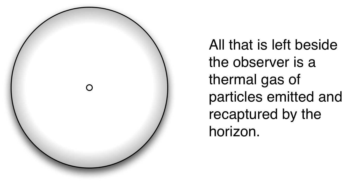
The Poincaré recurrence theorem says that eventually the current
visible universe would be recreated from the thermal gas. The recurrence time can be
enormously long though.
More modest fluctuations are also possible. A single solar system could
be created, or and Elephant.
Physicists apparently talk about Boltzmann brains being created this
way. A Boltzmann brain is a
minimal self-aware entity that pops into being as a result of random
fluctuations.
[
I found the following article on this topic
“Disturbing Implications of a Cosmological Constant” ,
Lisa Dyson, Matthew Kleban, Leonard Susskind
http://arxiv.org/abs/hep-th/0208013
]
Eternal Inflation
Another puzzle is known as eternal inflation. Sidney Coleman showed that de Sitter space is unstable. Small bubbles of space with a different and smaller cosmological constant continuously form.

Two different regions could eventually overlap. When two regions overlap, they may have different values for the cosmological constant. A domain wall would separate the values of the cosmological constant and we could possibly see a difference like a patch of sky that is too cold. People are looking for these differences in the cosmic microwave background. They could show up as a type of polarization of the microwave background.
The population of the bubble universes will exponentially increase. If each bubble had the same smaller cosmological constant, then they would all end up being the same size 1/H. They will fill up everything.
[Eternal Inflation
This looks like it might be a
good source. I haven’t read
it yet.
http://ebooks.worldscinet.com/ISBN/9789812832405/9789812832405.html
]
This leads to a probability puzzle:
1) The population is increasing exponentially
2) There are finite resources
3) The resource limit is unknown
4) The observer making the analysis is typical
5) What is the probability of lasting more generations
The answer is that the probability is that the end is near.
[Whatever
probability distribution you pick for the finite resources, there is a value
larger than 50% of the distribution. The end comes in log(limit)-log(current)
generations. I think the point
here is exponential growth is fast. In the case of de Sitter space I don’t see
why space can’t be created faster than the nucleation rate. The initial cosmological constant could
be very large. ]
Escher’s “Circle limit 4” is an interesting illustration. It is copyrighted so I won’t add it here. You can see a good picture at:
http://www.josleys.com/show_gallery.php?galid=325
There is a small copy at the top, but a much better/bigger copy about half way down the web page.
The “resources” here correspond to the room and resolution to accurately draw the features of the angels and devils. If you pick a “typical” devil and ask if it is completely drawn with all features, the answer is probably not. The vast majority of the devils are drawn on the edge of the circle at too fine a resolution for this to be possible.
A related problem is known at the “Measure Problem” [I imagine that this name is connected to the concept of a measure in the theory of integration.] The setup is that you have a infinite number of bubble universes with different values for some observable like the cosmological constant. You then ask what the expected value is for that observable. Any given value will appear infinitely many times, so you are dividing infinity by infinity which is nonsense. [I think the idea is that we would like to have an initial finite approximation based on a lattice or some other model. Then we can take a limit that hopefully converges to a finite answer. In the case of eternal inflation, there doesn’t seem to be an initial finite state to start with. ]
The lecture closed with a discussion of
the state of string theory. The
basic idea is that the String Theory that is well understood mathematically and
is Supersymmetric does not match the observed world. The theory needs modifications and extensions to
get there. The
mechanism to break supersymmetry is not known.
On the other hand, it is an existence
proof for the integration of gravity and quantum mechanics.
This was the last lecture in the
series. Professor Susskind
will be starting over in a future quarter. We can also look forward to a set of books corresponding
to the lecture topics.