Physics Notes: Supersymmetry,
Grand Unification, and String Theory
Lecture 1: March 29, 2010 Back to PHY31
Renormalization
Much of the quarter’s topics originate out of questions and puzzles associated with renormalization.
What is renormalization? Two parts:
How do we eliminate from our descriptions the behavior at very small scales, which also happen too fast to observe. [It seems like a kind of summarization of the overall behavior of the fine scale to be used in a theory at the coarser scale]
The second part is simply dimensional analysis. Dimensional analysis can be used in forming the summary of the fine scale.
Examples:
The nucleus at a fine level is made up of quarks, but for many purposes a model based on protons and neutrons is fine. So solve for and compute the properties of protons and neutrons based on QCD, then base the theory of the nucleus on that result. The properties could include mass, spin, charge, … . You will also need the forces generated between them. Then forget where the model came from and move on.
If you are interested in atoms (atomic physics) you may not be interested in protons and neutrons. You just have ~92 + isotopes nuclei with masses, charge, … . You also need to include electrons, which are very light with respect to the nuclei.
Molecules come next.
The same idea is true in QFT. All possible scales constitute degrees of freedom, many of which are at length scales outside of our range of interest. We want to summarize the contribution of the smaller scale degrees of freedom to simplify the model at the scale we are interested in. This together with dimensional analysis is renormalization
Example: Atoms to Molecules
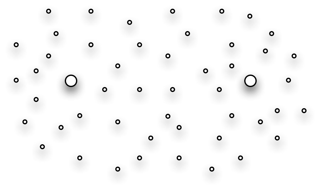
The Nucli are like bowling balls, very heavy and not moving fast. The electrons are moving very fast. We can separate the models by first treating the nuclei as a fixed background for the electrons.
Start with the Hamiltonian:

The first two terms are the kinetic energy of the two nuclei: a and b.
The third term is the electrostatic potential between the nuclei.
The part in [ ] is the contribution of the electrons, consisting of a first sum giving the kinetic energy of the electrons with the electrostatic potential with the nuclei, followed by a sum giving the electrostatic potential of the configuration of electrons.
There are two time scales, one for the nuclei, and one for the electrons. Start with the assumption that the two nuclei are in a fixed relative configuration and solve the electron problem for that configuration. The nuclei contribute only fixed parameters to the problem. Solve the Schrödinger equation for the lowest energy state – the ground state in the background of the nuclei configuration. Then replace the electron contribution in the Hamiltonian with that energy.
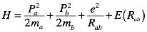
The last two terms are the potential energy contribution to the Hamiltonian and will look something like:
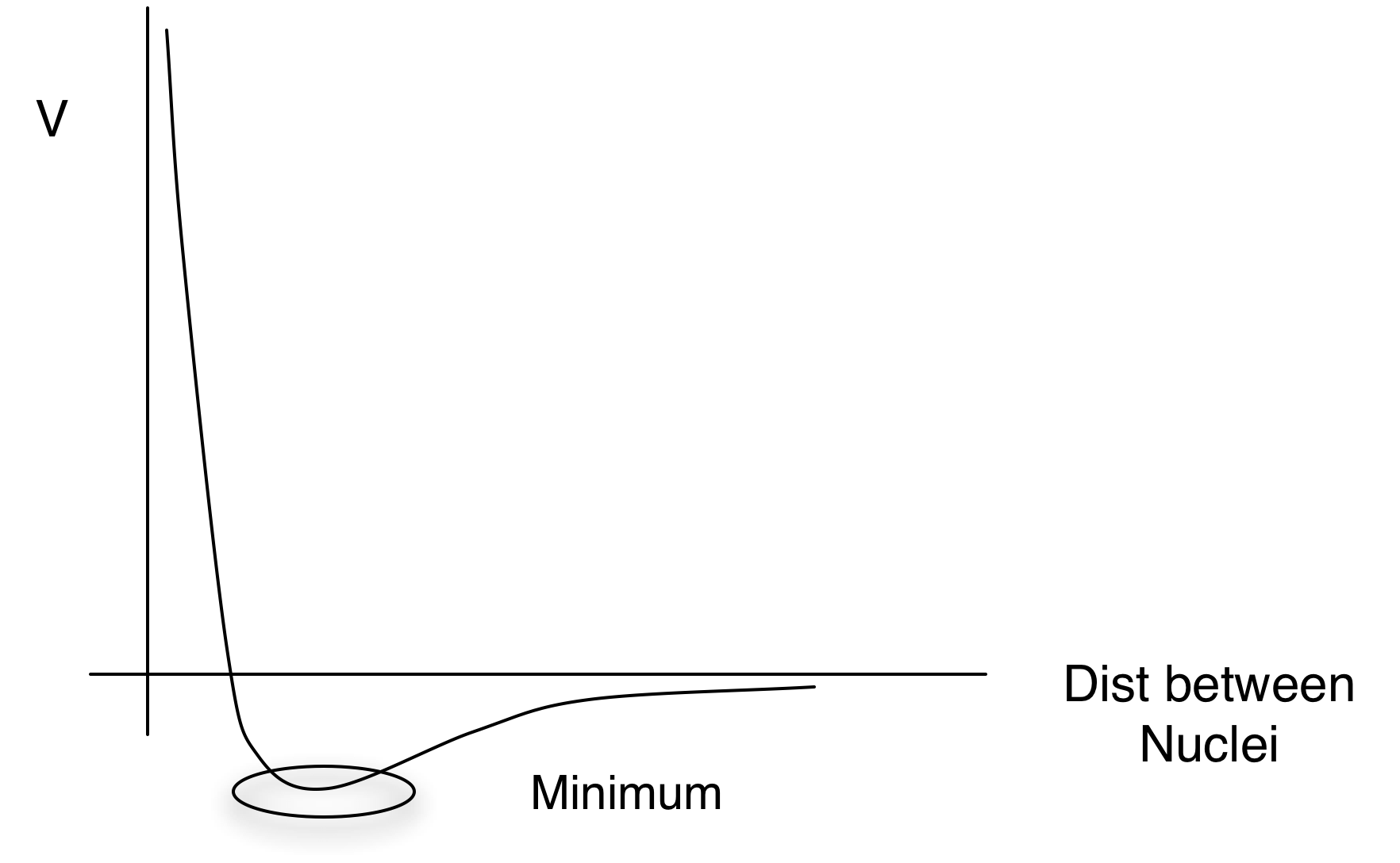
There is no need to think about the electrons. We have eliminated the high frequency degrees of freedom associated with the electrons from the problem.
Divergence in QFT
We have three related units: distance, time, and mass. If we fix  ,
then we have one. We can pick one
to work in. Length is a
common choice.
,
then we have one. We can pick one
to work in. Length is a
common choice.
Use [] to indicate the units of an expression.
[m] = [E] from E=mc2. We also have [E] = [P]
Also [L] = [t] = 1/[m]
Start with a Scalar QFT [The Higgs Particle]
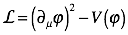 The first term being the
kinetic term.
The first term being the
kinetic term.
What are the units of the Action?
 (with units of
  ,
but we set that to 1 )
,
but we set that to 1 )
Since we are multiplying  with 4 directions of space-time, its
units must be:
with 4 directions of space-time, its
units must be:

So 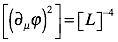
If we take a space derivative of  ,
the units are
,
the units are 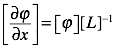
Squaring that we find that 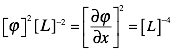
Finally: 
This helps us understand the potential function  .
.
A typical potential function:
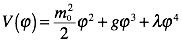
It is easy to see that [g] = [m] (units) and that  must be dimensionless.
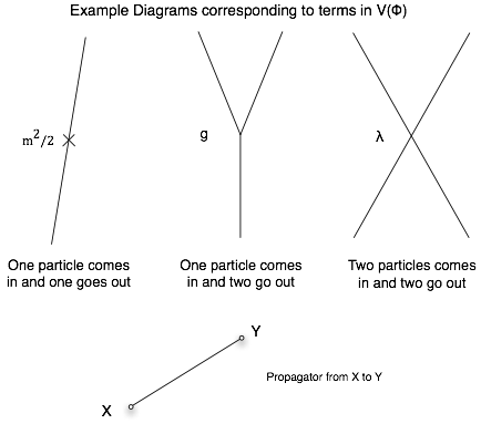
The coupling constant is not the whole story governing the amplitude for a graph. There are also propagators, which compute the amplitude for a particle starting at space-time point X to be observed at point Y.
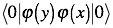 , which has dim [L]-2
The propagator represents an integral over all ways the particle can go from X to Y.
It has to be Lorentz invariant so a reasonable estimate is
 up to a constant factor.
Up close these propagators become infinitely large and are the source of all divergences in QFT.
Which takes us back to renormalization.
Renormalization in QFT
Do we really have to worry about propagators from X to X ( )? 10-17cm is small
enough for our low frequency purposes.
[physics probably changes below there anyway, so
pursuing the divergences to the bottom would be non-physical anyway]
)? 10-17cm is small
enough for our low frequency purposes.
[physics probably changes below there anyway, so
pursuing the divergences to the bottom would be non-physical anyway]
The idea is to find a process in nature that would mimic a
vertex. We can use our
graphs from higher order terms in V() with loops coming nearly back to the same
point. We pick a cutoff scale  for the analysis.
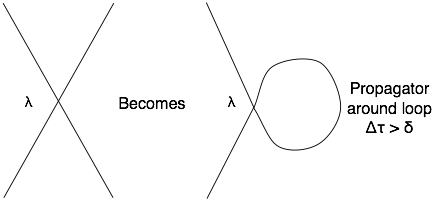
For the purposes of the propagator we blur the vertex out to
the cutoff scale  .
.
Now the combination of the loop propagator and  look
like the original mass term.
look
like the original mass term.

Our effective mass now includes contributions from higher order graphs with loops.
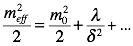
This is the mass seen in the lab at reasonable length
scales. Many other graphs
are possible. For example,
you can have a 2 vertex graph based on two joined copies of the same  graph.
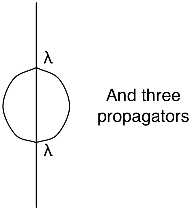
To analyze this graph we hold one vertex fixed and let the
other vertex vary over all space-time at distance greater than  .
.
The amplitude for this graph would look like:
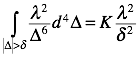
There are obviously infinitely many higher order graphs with
more internal vertices that generate contributions that are higher order in  .
Does this converge?
.
Does this converge?
What about the  term in
the potential? Once can easily
make a graph combining two corresponding vertices. It looks like the 2 vertex graph above, but missing the
middle line. The
integral form is a bit of a special case as it results in a log function.
term in
the potential? Once can easily
make a graph combining two corresponding vertices. It looks like the 2 vertex graph above, but missing the
middle line. The
integral form is a bit of a special case as it results in a log function.
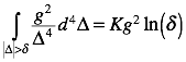 the ln() is dimensionless and
[g] = [m].
the ln() is dimensionless and
[g] = [m].
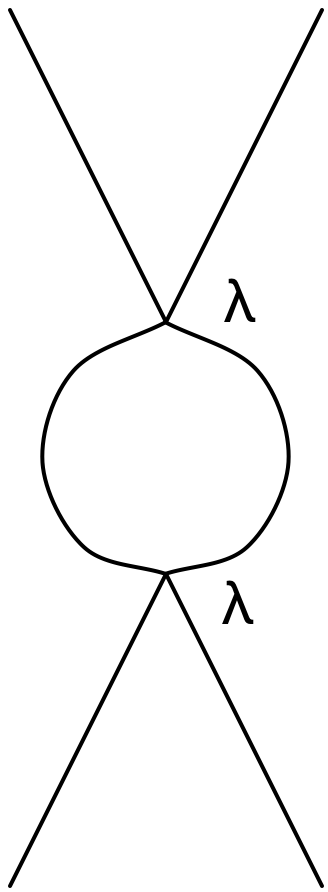
More than the mass gets renormalized. Every term gets
renormalized. The following
graph makes a contribution to  renormalization.
We need the generated series to cancel out to fine precision.
If we use  Planck length, then we have a sum of positive and
negative contributions each of which is 34 orders of magnitude larger than the
final result (which we know because of the assumed order of mass of the Higgs).
Planck length, then we have a sum of positive and
negative contributions each of which is 34 orders of magnitude larger than the
final result (which we know because of the assumed order of mass of the Higgs).
This is the mass hierarchy problem. Many big terms adding up to a tiny result – ridiculously fine-tuned!
Why are Fermions not a Problem?
The fermion mass term  exchanges left and right handed particles.
There are other couplings to a scalar particle (the Higgs for example – basically a particle that doesn’t change under rotation – spin 0). And there are the gauge boson interactions we studied last quarter.
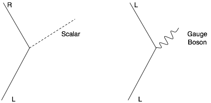
If a fermion had no mass, then there are no graphs with gauge boson loops that would contribute to mass because they wouldn’t change handedness of the fermion.
A scalar particle emission would change handedness, but the recapture of that scalar particle would flip the handedness back again. There are always an even number of such vertices.
The mass renormalization depends on having a mass to start with. Then you can have graphs like:
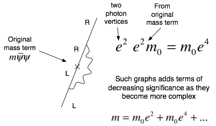
If gauge bosons start massless, they stay massless. It all boils down to the Higgs.
The Higgs is the only crazy fine-tuning problem in the standard model.
The next fine-tuning problem is gravity. This problem is caused by the renormalization of vacuum energy.
Normally energy differences are all that matters in physics. The source of gravity is Energy, not a difference in energy. Since the vacuum contains virtual particles, it has energy and it gravitates. The graphs that contribute are closed loop graphs with no input or output particles. While the Higgs requires fine-tuning to 34 decimal places, the vacuum requires about 123 decimal places, even crazier.
Supersymmetry may solve the Higgs fine-tuning problem by having particles appear with partners whose contributions cancel each other, but does nothing for gravity.
Question: The
selection of  seems
arbitrary. Does fine-tuning depend
on the value of
seems
arbitrary. Does fine-tuning depend
on the value of  ?
?
The place where the coupling constants converge seems like the right scale to use for now and corresponds to the smallest scale that we believe we understand the physics.
Question: How come the bose ground state doesn’t cancel the fermion ground state?
[This question appears to be in
reference to the scalar field example – the Higgs.]
It would still require a huge amount of fine tuning. The simplest diagrams for
fermions contribute negative terms and the simplest terms for bosons contribute
positive terms. However,
there are still the masses and coupling constants that all have to be balanced
out to high precision to leave a small mass behind. This is part of what Supersymmetry does, having
boson particles to go with fermions that have the right masses and coupling
constants to balance them out. [I think that’s a reasonable interpretation of the answer].