Physics Notes: Supersymmetry,
Grand Unification, and String Theory
Lecture 3: April 12, 2010 Back to PHY31
This lecture was short because of a seminar on the SLAC X-ray laser that started 1 hour into the normal period of Professor Susskind’s lecture. The notes are therefore also short. The main topic was more development of the notion of propagators. We covered a bit of propagators last quarter .
Renormalization of Mass
Feynman diagrams have several uses. One is to model scattering. They can also help with computation of the “effective” Lagrangian. We can remove complexity by using an energy or momentum cutoff. These are nearly equivalent notions of cutoff, different only in the rest mass contribution to energy, which is often very small.
Feynman diagrams contain propagators, which represent transporting a particle from one space-time location to another.
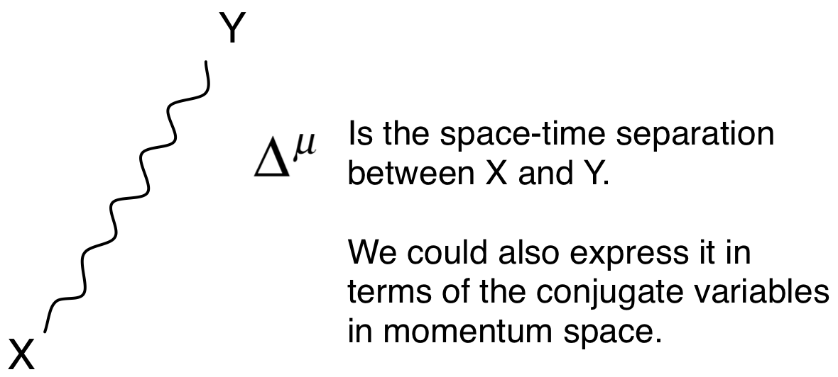
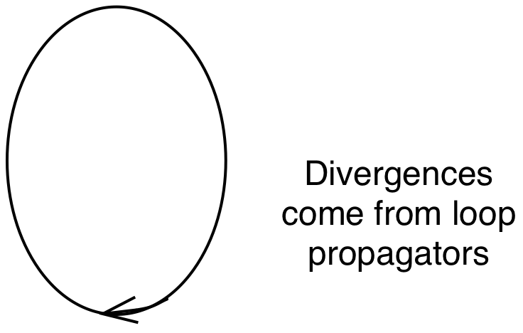
We integrate from a point back to nearby that point. For very small proper time
separations, the integral diverges and this is why we establish a cutoff. The integration is stopped inside
of a distance limit. We can
alternatively integrate across momentum space staying under a maximum
momentum. [The argument for such cutoffs seems to be that at these
limits, new physics appears which prevents the infinities from being real. We don’t know what that new
physics is, but we will just integrate across the domain we think we know and
hope for the best. ]
We have three basic particle types we have to worry about. Spin 0, Spin ½ and Spin 1.
The propagator represents a creation operation at Y and an annihilation operation at X. In general, all components of the field are represented.
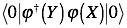 For a scalar
spin-0 particle
For a scalar
spin-0 particle
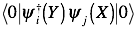 For a fermion.
In the fermion case both i and j are iterated through the components of the field, so the propagator is actually a matrix.
A general sense of what the propagator has to look like when evaluated can be had from dimensional analysis.
Remembering that the Action is dimensionless if we set  ,
we have
,
we have

So  must have units
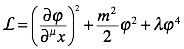
From the first term we can see that we have
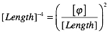
So
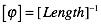
And therefore  must be dimensionless.
The Feynman graph representing the loop has two factors of  and two factors of
  from the propagator yielding units of
  which happens to match the units of the
mass term coefficient
which happens to match the units of the
mass term coefficient  . Given this we can expect the
propagator to have the form:
. Given this we can expect the
propagator to have the form:

Where K is some constant from the integration containing  like
things. At high
momentum (or equivalently, small distance) you can ignore the mass and this
form is pretty good.
Remember that:
like
things. At high
momentum (or equivalently, small distance) you can ignore the mass and this
form is pretty good.
Remember that:

If  ,
then the amplitude drops off rapidly. Something like
,
then the amplitude drops off rapidly. Something like

Applying this to graph for the  term, which looks like
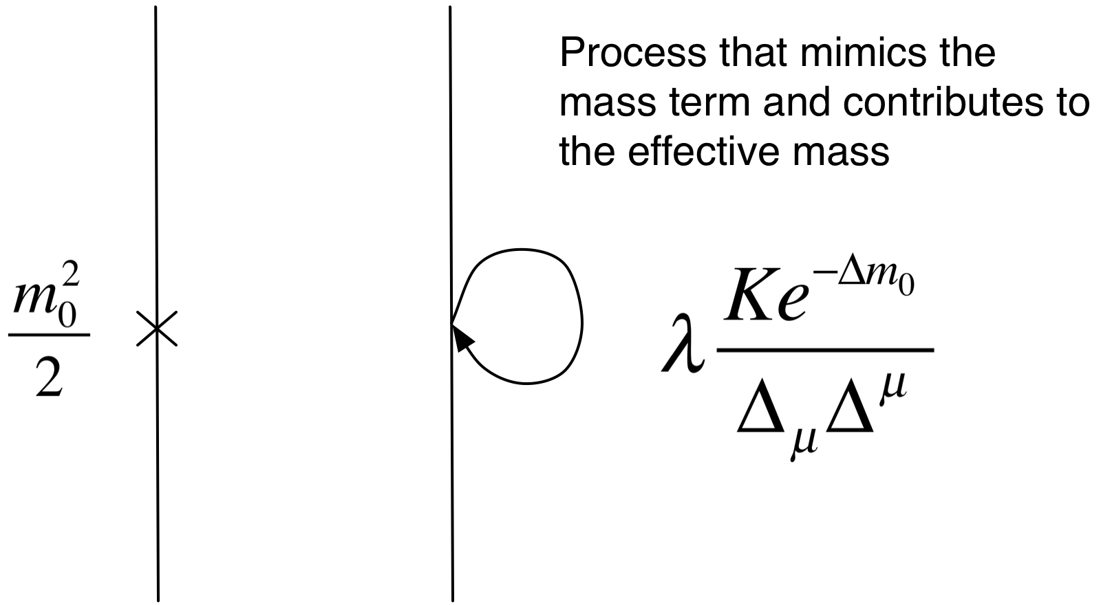
The graph on the right adds a
correction to the effective mass.
However, it makes an infinite contribution as  goes
to 0. This is where we
assume a fuzzyness on a scale of
goes
to 0. This is where we
assume a fuzzyness on a scale of  which is something like the Planck
scale. We either integrate
over spacetime and limit the interval to be far enough from zero, or we
integrate across momentum space and cap the momentum.
which is something like the Planck
scale. We either integrate
over spacetime and limit the interval to be far enough from zero, or we
integrate across momentum space and cap the momentum.
The renormalization
contribution to the effective mass can be larger than the base mass term  .
.
Fermions
Start with the action for a fermion:

It is easiest to figure out the units of the propagator from the mass term, but obviously you get the same answer either way.
If  and mass has units of
 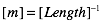 ,
then it must be the case that
,
then it must be the case that
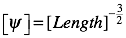
So the propagator would have units of .
Complicating things is that the field has 4 components, so the actual
form of the propagator looks like
.
Complicating things is that the field has 4 components, so the actual
form of the propagator looks like

This propagator is actually a matrix coupling the components
of  ,
in the same way as the mass term.
,
in the same way as the mass term.
The Sign of Fermion Loops
A pair of loops, either fermion or boson, will have a
positive contribution. If
the two loops are near each other, then there are two cases, either the
particles are exchanged in the loops or they aren’t. For bosons, these two cases just add to the
amplitude. For fermions,
when we exchange indistinguishable particles, we have to multiply by a phase of
-1 before adding. [There is an excellent discussion of this in the Dirac
lecture by Feynman].
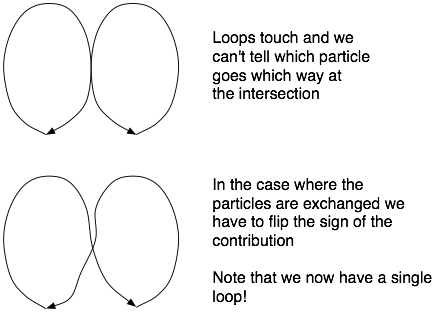
This alternate case where we exchange fermions must therefore have a contribution that is the negative of two separate fermion loops, which has the same contribution as two boson loops. But this is a single fermion loop! The implication is that individual fermion loops give a negative contribution.
If we suppose that bosons had a fermion partner with the same charge and mass, then we could imagine that the divergence in the renormalized mass would cancel out.
Fermion Loop Contribution to Scalar Renormalization
We can also have graphs with 3 edges connecting to a vertex. Two of these can be used to construct a second order graph using a fermion/anti-fermion pair loop to contribute to the renormalization of a scalar mass [Higgs].
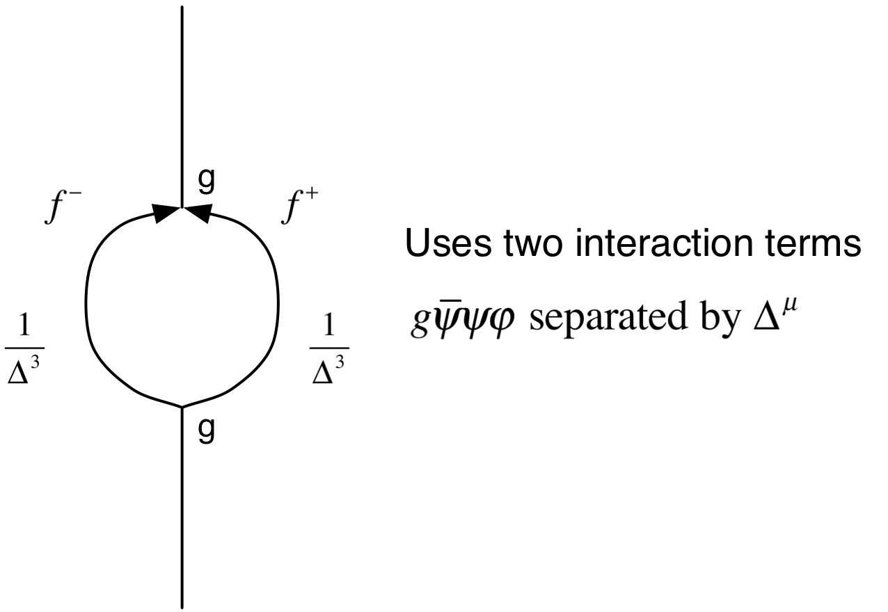
We still have to integrate over separations larger than  .
We can hold one point fixed and integrate over the displacement to the
other point.
.
We can hold one point fixed and integrate over the displacement to the
other point.
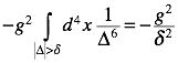
The minus sign comes from the fact that this is a fermion loop. Adding this to our previous contribution we get

We still need a miracle to get  .
.
This kind of miracle is what is posited in Supersymmetry.