Physics Notes: Supersymmetry,
Grand Unification, and String Theory
Lecture 8: May 24, 2010 Back to PHY31
Topics: Extending Supersymmetry to 4-space, Generated QFT, Feynman Diagrams
Questions
Q: Explain the FermiLab CP violation experiment and results
Particles and anti-particles are not a symmetry of nature. Looking around today we see lots of particles and not many anti-particles.
The experiment is based on collisions of protons and anti-protons moving in opposite directions.

The starting configuration is symmetric, but the result is not.
The collisions result in a bunch of junk + a muon pair, or equivalently a bunch of anti-junk + an anti-muon pair. If the starting condition is in fact symmetric, then one would expect that the rate of production of muon pairs and anti-muon pairs would be the same. They found an excess of muon pairs.
The standard model has CP (charge + parity) symmetry violation. Parity refers to reflection of all space axes. CP violation leads to a matter anti-matter imbalance in the universe. Imagine that the early universe had an equal and large number of protons and anti-protons. Most of them would annihilate with each other and you would have a lot of photons and an equal number of protons and anti-protons left. A small initial imbalance would therefore result in a large ratio between matter and anti-matter at the end.
The problem with the CP violation in the standard model is that the magnitude of the violation is about 10 times too small to account for the current ratio of matter and anti-matter. This new experimental result is much larger than the standard model predicts and is more consistent with the observed ratios.
The question this raises is, what is the source of the larger CP violation.
Q: Is there energy associated with the charge of a particle
Yes – there is energy associated with the field. However, if you take the case of protons and neutrons you might expect the proton to have more mass than the neutron.
Proton – uud 938.3MeV u is +2/3 charge, m=3.3MeV, d is -1/3 charge, m=6MeV
Neutron – ddu 939.6MeV
Why is the u lighter than the d? Charge would have it the other way.
This is not understood. Quark masses are just inputs to the model.
Lecture
In this lecture we will generalize Supersymmetry to 4 dimensional space-time, derive the associated QFT and corresponding Feynman Diagrams.
Start with a massless Fermion field. This will have two components:

There will be no term that mixes  with
with  , because that would create a mass term.
Let the Pauli matrices be:

We have stuck in a 0th component for time.
The Hamiltonian will look like:

Note that spin in direction of motion is positive energy; spin in the opposite direction of motion is negative energy. This leads to a compact equation form
 [looks like a continuity equation]
This is a Chiral Dirac Equation.
Note that the algebra of the Pauli matrices is anti-commuting except for the first one, corresponding to the time derivative, which commutes with the others.
Let’s form a two component field out of Grassmann numbers to go along with the generalization to space-time.
 Each component is a complex number
We can form the Q’s for each direction using this:

[Note the conjugation (transpose) of  .
I’m not sure if this is correct because it looks like we should get a -1
out of
.
I’m not sure if this is correct because it looks like we should get a -1
out of  since
it’s elements are imaginary. The
ordering of
since
it’s elements are imaginary. The
ordering of  is part of the transpose.]
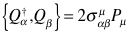
The commutator rules are:
The rest are:

Note that some rules are anti-commutators and some are commutators.
The Q’s and P’s correspond to small shifts in position because
they involve derivatives. [In the case of Q, the direction of differentiation is a mix of
a  direction
and a normal space-time direction. ]
direction
and a normal space-time direction. ]
The change in  , the superfield, in the Q direction is then:

We can also apply a constraint to the superfield, which reduces the number of independent components. As we saw in the previous lecture, as long as the constraint commutes or anti-commutes with the generators of the symmetry, then the constraint is compatible with the symmetry.
A constraint that works is:
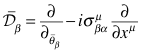
What does this constraint do? Another way to ask this is which variables does it remove? Let
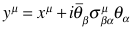
Then



This implies that we can remove  .
.
If we expand the superfield into components, there are only 3:

The last term is not 0. It really represents products of pairs of Grassmann variables.
Now y is not x, eventually we have to translate back.
The Action
Suppose we have a simple Lagrangian term:

We need to integrate this across all the  space. A
trick we can use when performing a complete definite integral is that we can
add an offset to the integration variable. We can change the integrand to:
space. A
trick we can use when performing a complete definite integral is that we can
add an offset to the integration variable. We can change the integrand to:
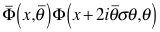
Expanding:





Remembering that we only need the terms with all the Grassmann variables because they are only ones to survive integration:
=
 This
part is the Klein-Gordan scalar term
This
part is the Klein-Gordan scalar term
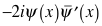 This
is the massless Dirac fermion
This
is the massless Dirac fermion
 And
what is this?
And
what is this?
The first two terms involve derivatives corresponding to small changes in positions or velocities (momentum) and correspond to standard propagators. The last term corresponds to a propagator that takes out a particle and puts it right back at the same place. On the face of it this seems useless [– but wait …].
A key event here was that the original Lagrangian had no derivatives, but now we have them. They came about via the Taylor series expansion of the components of the superfield. This looks promising but too simple. What about mass terms? Let’s try a different Lagrangian term. In this case the input shift for integration gets rid of the complicated terms completely.

Keeping only the terms that contribute to the action (and using a
special case that wasn’t explained, where we only integrate across variables appearing
in the integrand.
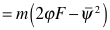 Minus sign for
swapping Grassmann var to end.
Minus sign for
swapping Grassmann var to end.
The second part of this is known as a Majorana mass term. What about the first term? Remember that an F creates a particle that doesn’t go
anywhere in space-time.
However, the F can turn back into the  . The composite
graph would look like:
. The composite
graph would look like:
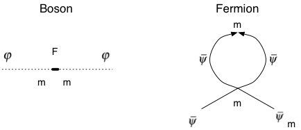
In the graph on the left it looks like a coupling from a
boson to a boson with a coupling constant of  .
The graph on the right is also a composite graph with two factors of
m. In this way the fermions
and bosons get the same masses.
It turns out that every boson graph has a dual fermion graph and since
bosons and fermions make opposite contributions to the vacuum, they cancel out
completely.
.
The graph on the right is also a composite graph with two factors of
m. In this way the fermions
and bosons get the same masses.
It turns out that every boson graph has a dual fermion graph and since
bosons and fermions make opposite contributions to the vacuum, they cancel out
completely.
Supersymmetry is establishing relationships between coupling constants for bosons and fermions.
Suppose that we add a new term with a new coupling constant to the Lagrangian

The important terms in the product are:
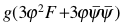
Notice that the coupling constants for the Feynman graphs for bosons and fermions are locked together.
To come: Symmetry breaking for Supersymmetry and Unification with SU(5)